Article: The Evolution of Definitive Screening Designs from Optimal (Custom) DoE
Part two of a series of three articles exploring Practical (Real-life) Implementation of Sequential Design of Experiments and the Introduction of Definitive Screening Designs
Written by Dr. Paul Nelson, Technical Director.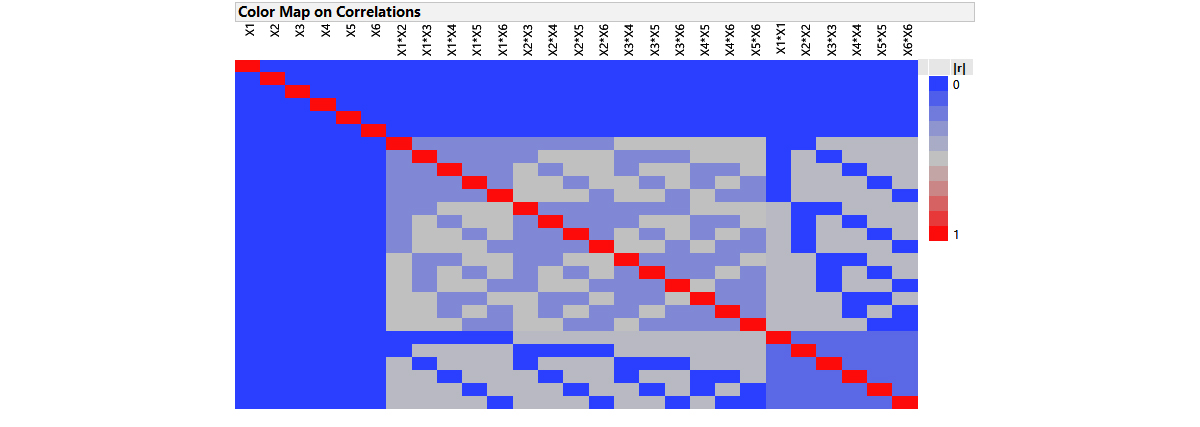
Optimal (Custom) designs implement the idea of model-oriented design. That is, they maximise the information about the specified model, you deduce a priori, to fit to the resulting data, whereas the classically designed experiments described in my previous article The Sequential Nature of Classical Design of Experiments often have strong combinatorial structure, or symmetry, such as orthogonal columns. This suggests the analysis of these classically designed experiments profits by taking advantage of what is already known about their structure: design-oriented modelling.
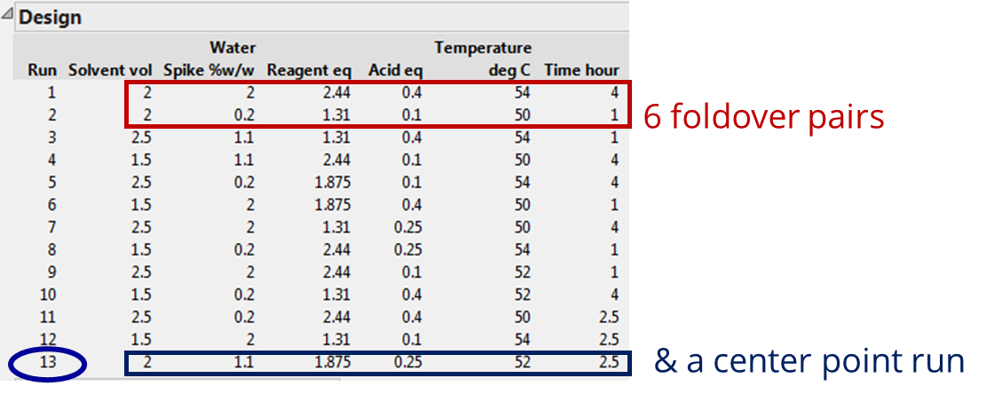
Definitive screening designs (DSDs), introduced by Jones and Nachtsheim (2011), have a special 3-level, fold-over and alias-optimal structure with many desirable combinatorial properties in addition to being resource efficient [1]. The DSD for the 6 continuous Esterification parameters is displayed below. Note that the rows of the DSD in standard (unrandomized) order illustrate the fold-over pairs of runs which mirror each other and result in a design that has twice the number of runs as there are factors, plus one centre point row where all the factors are at their middle setting. That’s just 13 runs. Recall, for the classical 2-level fractional factorial screening study discussed in the previous article, the number of experiments came to 20, but we still had to augment a further 6-10 runs to model the curvature and response surface around the optimum in detail.
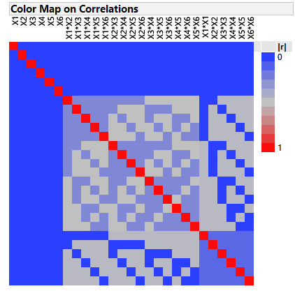
The fold-over structure of DSDs results in orthogonal main effects, and main effects are also orthogonal to all second-order effects. The colourful correlation cell matrix below emphasises these particularly desirable properties. Desirable, because screening designs are primarily intended to support first order models, but there is often concern that responses might exhibit strongly curved behaviour over the factor ranges. This might lead an investigator, using a classical 2-level screening or fractional factorial design, to falsely screen out a factor as having no (linear) effect when in fact it is important to the process. It is for this reason that DSDs are called Definitive. The ability to estimate quadratic terms for and attribute curved as well as linear behaviour to the factors under study.
It should be re-emphasised that screening is not about optimising factors, but primarily about screening for the vital few factors to take forward to a full characterisation or optimisation step. Due to their special structure however, DSDs can project to highly efficient response surface designs in the presence of sparsity in the number of active factors. In other words, they can reduce the likelihood of having to augment your screening design to support a more complex model needed for optimisation, as we previously had to do in the case of the classical optimisation RSM design study here. There is one pair of runs where each factor is at its centre point and, together with an additional run where every factor is at its centre point, so that DSDs with more than five factors project onto any three active factors to enable efficient fitting of a full RSM model.
13 runs to estimate the 28 full RSM model terms just doesn’t go! As stated above, the minimum number of runs required to estimate the 28 terms: 1 intercept, 6 main linear effects, 6 quadratic terms and 15 2FI terms is 28. The minimum number of runs to estimate all main and quadratic effects together with the intercept term in this case is 13 runs. A design whereby you wish to estimate as many terms in a model as there are runs is said to be saturated. If there are more terms in your model than runs, as in this case, then the design is supersaturated. However, consider the sparsity assumption; the orthogonal structure of DSDs and later an analysis which exploits this structure, then there is potential to do more with less.
Wow, DSDs, with their desirable combinatorial structure, look extremely useful and resource efficient alternative designs to the classical 2-level screening designs we described above. Since both authors of DSDs are leading practitioners and proponents in the optimal design of experiments, it might not come as any surprise to learn that DSDs in fact started life as alias-optimal[2] designs. Perhaps at first it would therefore appear fascinating that DSDs have such a balanced, practical and appealing combinatorial structure. However, balanced orthogonal combinatorial designs are also optimal and Xiao, Lin and Bai (2012) showed that the combinatorial properties of Conference matrices meant that the construction of a DSD was both immediate (i.e., not requiring a computerised search for a global optimum design solution), but also straightforward.
As screening designs, we have learned that DSDs have many desirable properties. Lets recap:
Main linear effects (MLEs) are orthogonal to each other and are orthogonal to two-factor interactions (2FIs) and quadratic effects (i.e., 2nd order terms).
No 2FI is confounded with any other 2FI or quadratic effect although they may be correlated.
For DSDs with 13 or more runs, it is possible to fit the full quadratic model in any three-factor subset and regardless of which three factors, all the quadratic effects of the continuous factors are estimable.
DSDs can accommodate a few categorical factors having two levels.
Blocking DSDs is flexible. If there are k factors or parameters, you can have any number of blocks between 2 and the number of factors (k).
DSDs are inexpensive to field requiring only a minimum of 2k+1 runs.
You can also add runs to a DSD by creating a DSD with more factors than necessary and dropping the extra factors, which are referred to as ‘fake’. The resulting design has the first five properties above, with the bonus of more power and ability to identify more second-order effects.
The above characteristics often make DSDs the best choice for any screening experiment where most of the factors are continuous and particularly if resource and material is at a premium.
The analysis of DSDs often employ generic regression methods, which do not take advantage of all the useful structure DSDs possess. However, the analytical approach for DSDs proposed by Jones and Nachtsheim (2017), does take explicit advantage of the special structure of DSDs. Specifically, it uses the fact that first (main linear) and second order (2FI and Quadratic) effects are orthogonal to, or independent of, each other and splits the data into two orthogonal columns[3], and consequently, the analysis into two parts. Part 1 identifies the active main linear effects. Part 2 investigates all subsets of only those 2nd order terms containing the active main effects – referred to as obeying the heredity assumption. The effects listed in the two parts are finally combined to provide one model and analysis.
The randomised minimum run DSD for the Esterification case study is displayed below together with the two-part and combined analysis of the product data.
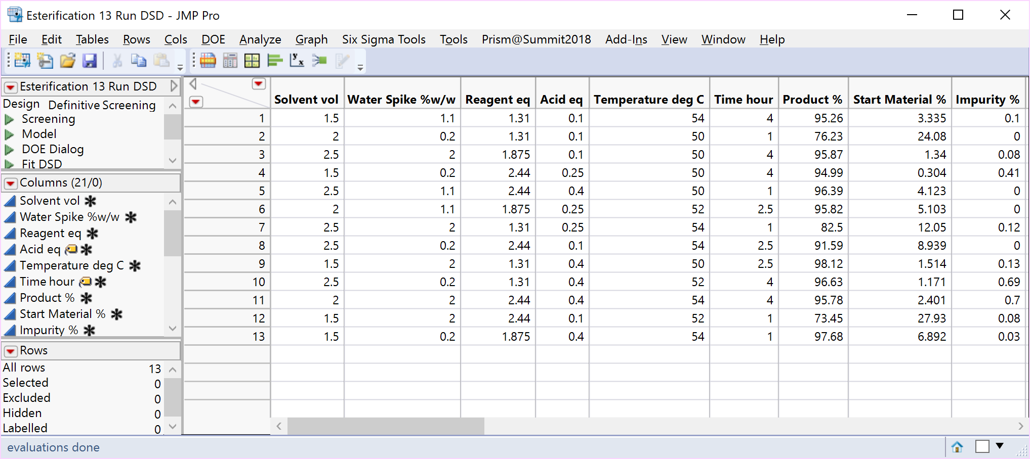
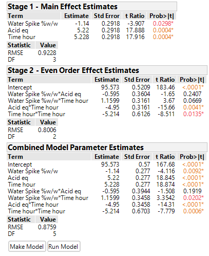
The same critical parameters, Acid and Time, appear together with the less significant water spike. Since the full RSM model for any three factors is estimable and only three factors have been shown to be significant, the DSD in this case has avoided the need for further experimentation (i.e., an additional optimisation step).
***
[1] A minimum run DSD is saturated by the main or linear effects and quadratic effects of the continuous factor and supersaturated if you include all second order terms (i.e., the addition of two factor interactions, or 2FIs, into the model).
[2] Alias Optimal designs protect main effects from bias introduced by the inclusion of 2FIs in the model
[3] By fitting a model including all the MLEs and excluding the intercept. The predicted Y values (YME) will be used to identify the MLEs in part 1 and the orthogonal, or uncorrelated, residual Y values (Y2nd) used to identify the 2nd order effects in part 2.
References
Jones, B. J., & Nachtsheim, C. (2011). A class of three-level designs for definitive screening in the presence of second-order effects. Journal of Quality Technology, 43(1), 1-15.
Xiao, L., D. K. J. Lin, and F. Bai. (2012). Constructing definitive screening designs using conference matrices. Journal of Quality Technology, 44, 1–7.
Jones, B., & Nachtsheim, C. (2017). Effective Design-Based Model Selection for Definitive Screening Designs. Technometrics, 59(3), 319-329.
This is the second part of a series of blogs exploring the Practical (Real-life) Implementation of Sequential Design of Experiments and the Introduction of Definitive Screening Designs. This article follows The Sequential Nature of Classical DoE, and precedes Strategies to Combat Problems Employing DSDs.
For more information about how Prism Training & Consultancy can assist you with statistical support, please click here to contact us and learn more about our services.
Be the first to know about new blogs, upcoming courses, events, news and offers by joining our mailing list here.