Article: Statistical Analysis of Equivalence Data from Method or Technology Transfer Studies

Following the steps in part one and two of this series of statistical articles exploring Method or Technology Transfer, it's now time to analyse our data, assuming we have adopted a nested design.

Following data collection, statistical analysis will provide:

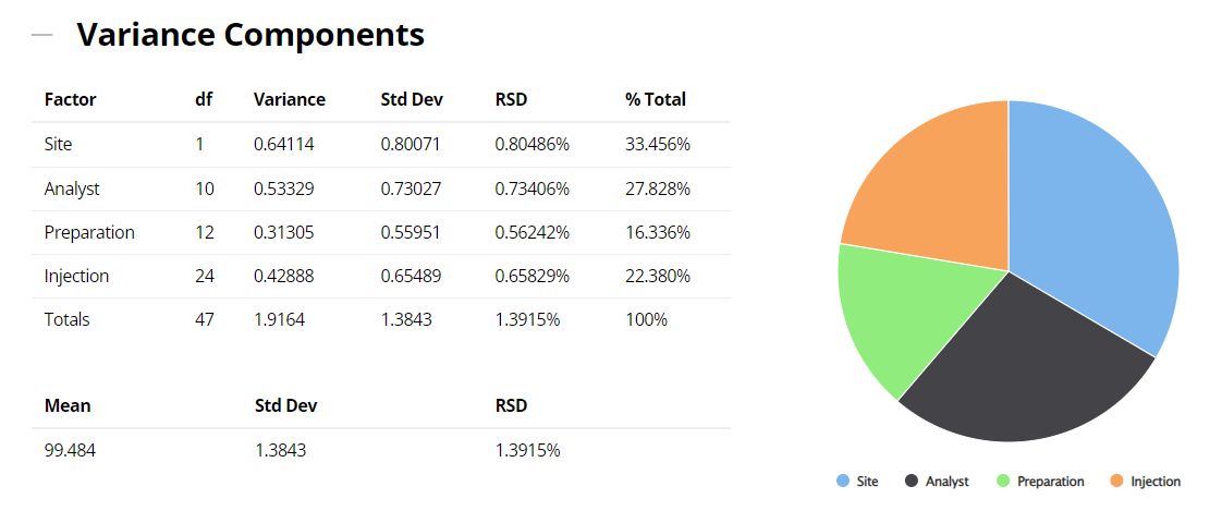
1. Estimates of variation contributed from each source separately (these isolated estimates of variance are called variance components and the statistician will speak of a “variance components analysis”);
2. Standard deviations and RSDs representing the three levels of ICH precision: repeatability, intermediate precision and reproducibility;
3. Difference (bias) between sites together with the standard deviation, confidence interval and TOST for the difference between sites to assess equivalence
4. Opportunity to evaluate, verify and forecast the variability of the data collection, assay format or replication scheme (design) for future studies and to meet future acceptance criteria

1. Variance Components: the variation in the data resulting from a nested study can be conveniently displayed in a dot frequency plot. The vertical axis in Figure 1 corresponds to the assay or Label Claim (%) response. The horizontal axis is defined as the combinations of the levels of the sources of variation. Data are then enclosed in rectangles to highlight the variation from each of the sources.

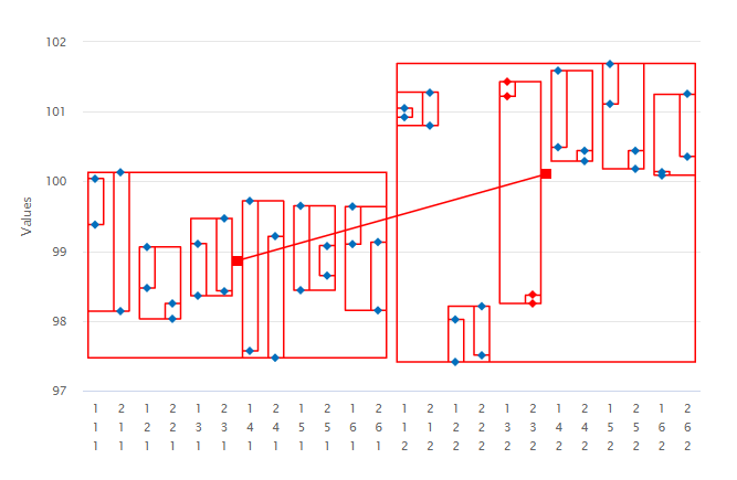
When contemplating a method transfer with different sites and potentially many analysts or operators performing several preparations on different occasions and repeat injections of each solution, all these sources of variation will be in operation. In the above example therefore, it is important to isolate and quantify all four variance components: site, analyst, preparation and injection (s_s², s_a², s_p² and s_i²). The sum total of these sources incorporates and characterizes the nature of both inter- and intra-site contributions to the technology transfer. The results of the variance components analysis are reported below.

2. ICH Three Levels of Precision Summary: using the variance components estimates above, the reproducibility (Site variation); the intermediate precision (sum of the Analyst and the Preparation variation); and the repeatability (Injection variation) can be determined and displayed.

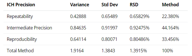
Figure 3: ICH Three Levels of Precision Summary from a Method or TT Study [1]

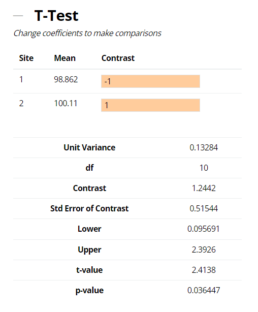
3. Assessing Equivalence: as we explained at the beginning of this article/series of blogs the traditional Student’s t-test or ANOVA approaches – testing for ‘zero-difference’, or no bias, when comparing the data produced by two or more sites – looks for evidence of a difference. Small variability (good precision) from the sites can mean that even small differences in the site averages, which may be of no practical significance, can be shown to be statistically significant.

In the example shown below, a difference (bias) in means of 1.2442% (100.11 – 98.862) between the Manufacturing Operations and R&D sites contrasted with a zero difference is 1.2442%. Comparing this to the standard error of the difference; derived from a weighted sum of the other, within-site, sources of variation and their respective sample sizes (see Equation 3 below), leads to a t-value or signal-to-noise ratio = 2.4138. This in turn results in a p-value (i.e., a risk assessment of you being right when you say there is no difference between sites) = 0.036. This is small, so the hypothesis of zero-difference is rejected and the method would be deemed to have failed the technology transfer by this approach.

However, if the objective of a technology transfer is to provide evidence of equivalence, rather than evidence of a difference, Lung et. al. [2] suggest that “a more appropriate statistical question is to ask…is there an unacceptable difference between two sets of results?” Instead of testing a zero-difference null hypothesis (i.e., there is no bias between the means), Lung et. al. recommend testing the more appropriate null hypothesis: there is a bias between the means larger than that which is considered a practically “acceptable difference”.

The general concept of comparing methods, including testing for equivalence, is proposed in the USP<1010> chapter ‘Analytical data-interpretation and treatment’ in the USP Pharmacopeial Forum [3] [4]. Guidance on setting appropriate acceptance criteria for a technology transfer is given in the section on Acceptance Criteria below. For illustrative purposes, suppose that a reasonable ‘acceptable difference’ limit between the two sites is ±3%.

More than one equivalence testing method is available, but the one recommended in this text is the Two One-Sided Test (TOST) proposed by Schuirmann, as it is simple to implement and intuitive. It uses two (lower and upper) one-sided t-test calculated from the difference between site means contrasted not with a zero difference, but with the pre-specified respective lower and upper acceptable bias or difference limits (equivalence margin). For this reason, results from the TOST are commonly expressed in terms of a confidence interval. If the classical (1-2α) confidence interval (e.g. if α = 0.05, then 1-2α = 90%) for the difference between sites is within the acceptable difference limits, then the hypothesis that the bias is greater than that which is considered acceptable is rejected and the sites can be concluded to be equivalent.

In our example, the difference (bias) in site means of 1.2442%, together with the traditional t-test, acceptable difference and TOST expressed as lower and upper 90% confidence limits are provided in output above. Since the 90% confidence interval for the difference (bias) between the two sites is enclosed within the ‘acceptable difference’ of ±3%, then per the TOST approach we can conclude that the data from the two sites are in fact equivalent for the method transfer.

Note that the tests and confidence intervals described above are appropriate when determining any statistical difference or equivalence in accuracy. Equivalent techniques are available for comparing the precision between two sites and are based on the F-statistic (ratio of variances).

For methods that have high variability e.g. moisture determination in some cases, or the quantification of extractables and leachables, a direct comparison of the means and RSDs for analyst, instrument and laboratory can be considered. This approach relies on a comparison of both the bias observed between the two laboratories and the variability observed in the receiving laboratory, as well as the overall RSD up to the limit values (acceptance criteria). This is the ‘descriptive approach’ to comparing data from two sites.

4. Sample size: a question frequently asked is “How many replicates are needed for a validation or TT study?” To develop a strategy to answer this question, consider the variance of an average result calculated from a single site involving m analysts, n preparations and k injections per preparation -

Equation 1:

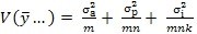
If estimates of these variances are available from a variance components analysis, as in subsection 1 above, then re-writing Equation 1 first in terms of RSDs -

Equation 2:

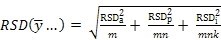
... and then in terms of the standard deviation of the difference between two sites employing the same replication scheme -

Equation 3:

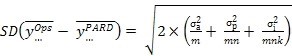
This enables the choice of the number of analysts (m), preparations (n) and injections (k) to achieve final goals either in terms of an acceptable RSD using Equation 2, or a least acceptable difference using a confidence interval derived from Equation 3, or both.

***

[1] Intermediate Precision (IP) expresses intra-laboratory variability and commonly incorporates repeatability. In the example, the IP variance, standard deviation, and %RSD would equal 1.27, 1.13, and 1.0% respectively.

[2] Lung, K. R. Gorko, M. A. Llewelyn, J. and Wiggins, N., Statistical method for the determination of equivalence of automated test procedures. Journal of Automated Methods & Management in Chemistry, 25 (2003), no. 6, pp. 123-127

[3] Pharmacopeial Forum, 27 (2001), 3086.

[4] Pharmacopeial Forum, 29 (2003), 194.